In short…
In OldInsuranceMaps.net it is now possible to georeference maps with only two ground control points, instead of the previously required three. For the time being though, we’re keeping this capability hidden (more about that in this discussion and below), but I wanted to write a good summary here of how it works and why it is beneficial. Thanks to Dan VK for requesting this functionality in a Github ticket, and helping out along the way to streamline some of the code. I’d been wanting to try to figure this out at some point, so this was a good push in the right direction.
GCPs + transformation algorithm -> warped map
To georeference a scanned historical map, you must create ground control points (GCPs) that link locations on the map with real-world coordinates. Then, these GCPs are fed through a transformation algorithm which results in a warped image. The QGIS documentation has a good summary of the most common algorithms, including those mentioned below.
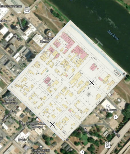
With three or more GCPs, OIM defaults to using the Polynomial (1st order) (a.k.a. “affine”) transformation, which rotates and skews the image to match the control points while still retaining the internal integrity of the original document. The example below shows this, with three good GCPs and one bad one (in blue) added to cause the image to skew for illustrative purposes.
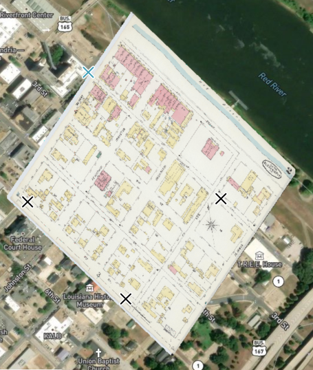
OIM also supports the Thin Plate Spline transformation, which will mush the map every which way to make it fit any GCPs you give it. Consider how the same map and GCPs from above produce a very different and much more distorted warped output when you use Thin Plate Spline.
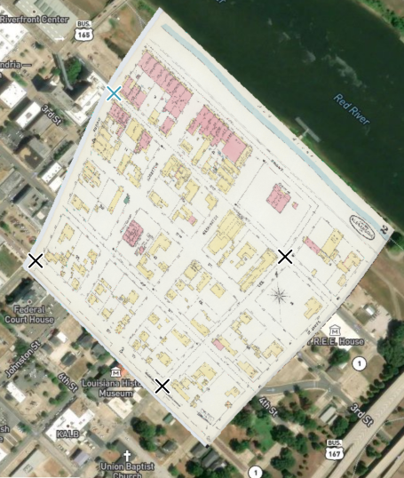
However, these two transformations require three or more GCPs, but now a third transformation, Helmert, can be performed with only two (this is the new thing!).
Why is this good?
Well, it’s not always possible to create three GCPs that are well-distributed across a page, because some split map pieces are too small, or only have linear features, or are in areas that have changed too much since the map was drawn.
Here’s a good example in the form of a warehouse in Alexandria, La., from 1896:
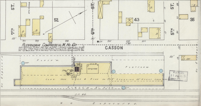
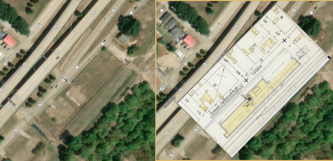
There are three intersections here, Casson with 5th, 6th, and 7th streets, but they are all in a row which is not helpful for Polynomial or Thin Plate Spline. But, using just two of these intersections with the Helmert transformation we can get a good fit:
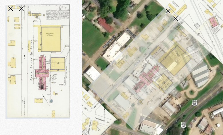
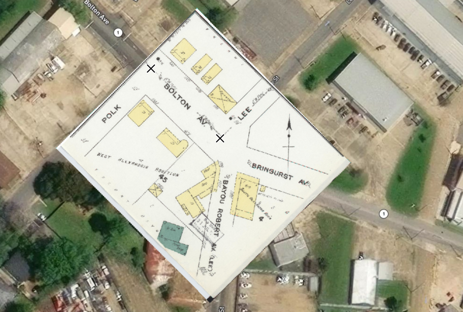
Going further, we can combine Helmert with a reference layer of adjacent georeferenced layers to get some pretty impressive (if, perhaps, questionable??) stitching. To illustrate, in the following image the upper layer has already been georeferenced, and we are looking to georeference a new layer below it. But the area of the layer has no good GCP matches when looking at today’s aerial imagery or street map.
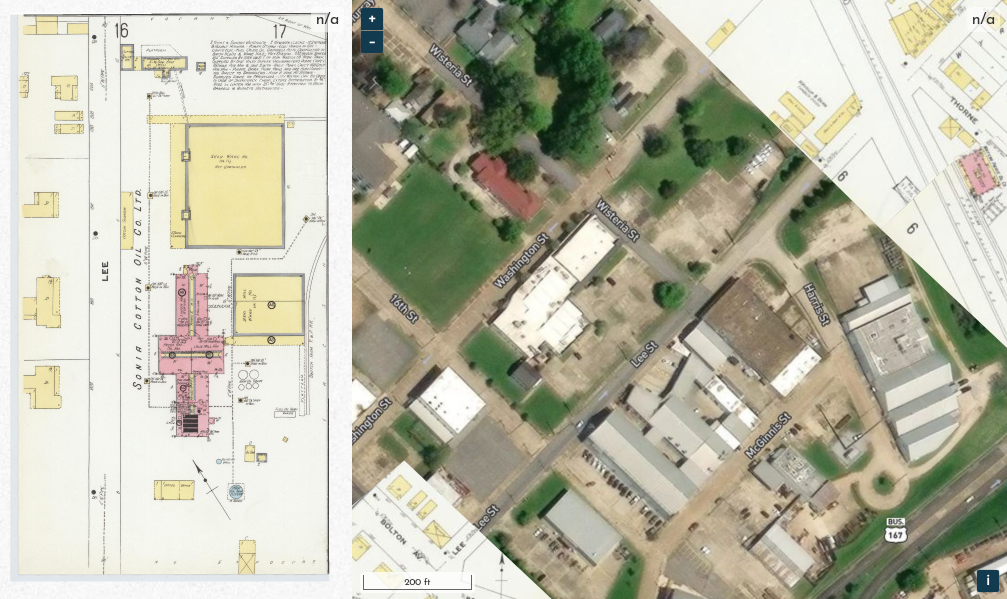
However, as is fairly common with Sanborn maps, on the bottom edge of the upper layer there are buildings outlined that are also represented on the layer we are looking to georeference. We can make two GCPs based on these overlapping building corners.
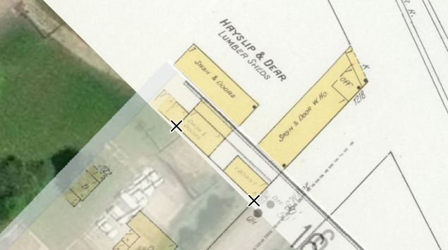
Even though these are only two GCPs, tucked away in the top corner of the image, using Helmert they are enough to allow us to georeference the entire map as it lays out down the street.
Pretty cool! This would be especially helpful in places where there has been significant urban development, or on the edges of small towns where old sawmills have returned to being forests.
Just because we can, does that mean we should?
For now, we are keeping Helmert somewhat hidden in the interface, and this is mainly because if you only use two GCPs, it’s easy to make something very quickly that may look good at first, but would actually be greatly improved by even one or two more GCPs and use of the Polynomial transformation. Also, it can be very finicky because, considering an example like that shown above, even very small adjustments on one of the points will cause big swings in the location of content on the far side of the page.
But I think it’s worth exploring further and making more accessible, so, if you have thoughts about this or opinions on best practices for georeferencing, we’d love to hear them! Add to this Github discussion, or join us on the OpenStreetMap US Slack in the #oldinsurancemaps channel, where we’ve talked about this a bit already.
The rest of this post will go further into how it all works anyway.
“Feels like witchcraft” – WallyKitty
Implementing the Helmert transformation was more challenging than I expected it to be. OIM uses GDAL’s Python bindings on the backend, which (essentially) take in GCPs and allow you to specify which order of polynomial to use, or alternatively to use thin plate spline. Then, a warped image is produced. Easy.
But there is no switch to flip to tell GDAL to use Helmert, so I had to create a custom proj pipeline instead and pass that to the warping operation. That pipeline is where you provide Helmert its four parameters, so once the plumbing was set up to get the pipeline working, it was time to figure out how to calculate those parameters, based on two input GCPs.
Each GCP is a linked set of two coordinate pairs, one is the x, y pixel location on the original image in pixel space, and the other represents the latitude/longitude of a real-world location in coordinate space. More specifically, coordinate space is the projection you are using (in this case, Web Mercator), so another way to think of it is that there are two flat grids, one is the original image where each pixel is represented by an x,y coordinate, and the other is the target map projection.
By comparing the values of the two GCPs, we need to come up with the following parameters, which the Helmert transformation will use to transform pixel space into coordinate space:
- scale: A scale factor applied uniformly to the image.
- rotation: How far around the image will be rotated.
- x offset and y offset: The target location in coordinate space of the top-left corner of the image.
If you understand that these parameters are all that Helmert needs, it’s not actually so hard to visualize exactly how the transformation takes place:
- The image is scaled up or down so that it is the right size. If, for example, on the scanned historical map there is a scale bar that marks 100 meters, and this scale bar is 50 pixels long, then the scale factor would be 2, so that 1 unit in pixel space represents 2 units in coordinate space (in our target projection, the units are meters).
- The image is rotated. If the original image shows north going toward the top of the page, then no rotation is necessary. But if north points to the left on the original image, it must be rotated 90 degrees clockwise.
At this point, we can imagine the image would be properly resized and rotated but without the final two parameters it will remain stuck at 0,0 in coordinate space. In the Web Mercator projection, 0,0 equates to latitude = 0, longitude = 0, or null island off the western coast of Africa. So…
- Lastly, the x, y offsets need to be calculated to tell the transformation where to put the top-left corner of the image. Now it is scaled, rotated, and shifted, so it appears in the correct location. All based on just two GCPs!
Originally, I calculated each of these parameters one by one with some math and trigonmetry that would have made my high school math teacher proud. But there were a couple of limitations with how I had set things up, and after I added some tests, Dan VK contributed work that simplified the logic significantly by using a single numpy function instead of all the individual calculations. Turns out this one function returns everything we need!
Overall, even beyond the immediate benefits that this particular transformation bring, this was a very worthwhile foray into some of the more nitty gritty aspects of georeferencing and transformations, and I look forward to working on more improvements like this in the future.